The Problem of Heterogeneous Supply Signals
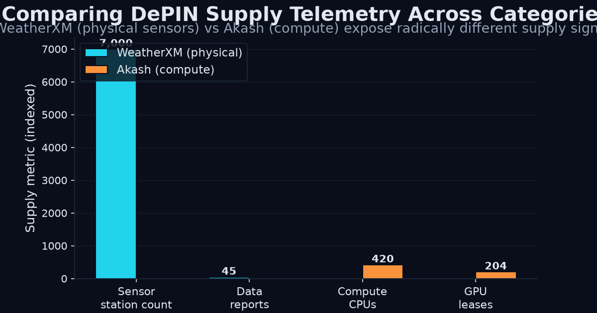
Decentralized Physical Infrastructure Networks (DePINs) expose radically different supply-side telemetry depending on their resource category. A wireless sensor network like WeatherXM emits station count, geographic coverage, and data-quality metrics. A compute marketplace like Akash emits active leases, CPU/GPU core allocations, and provider uptime. Naively comparing "3,000 nodes" across these networks is meaningless—you're conflating a $120 weather station with a 64-core GPU server.
The solution requires a canonical telemetry schema that normalizes heterogeneous supply signals into commensurable units, paired with self-certifying verification URLs that allow any observer to independently audit the claimed state. This post derives that schema and applies it end-to-end.
---
Supply Telemetry: Raw Signal Decomposition
WeatherXM: Wireless Sensor Network Telemetry
WeatherXM operates a network of LoRaWAN-connected weather stations that publish atmospheric readings on-chain. The core supply telemetry is exposed via their REST API and on-chain state.
Station Registry State:The on-chain station registry maps a station ID to a metadata struct:
struct Station {
    station_id: Bytes32,       // keccak256(mac_address, model_hash)
    owner: Address,            // staking wallet
    lat: i32,                  // latitude * 1e6 (fixed-point)
    lon: i32,                  // longitude * 1e6
    elevation: u16,             // meters
    model: StationModel,       // WS1 | WS2 | WS_PRO
    last_heartbeat: Timestamp,  // unix epoch seconds
    total_observations: u64,    // cumulative on-chain data submissions
}
The key supply metrics WeatherXM publishes are:
stations_registered — Total stations ever registered on-chain.stations_active — Stations with last_heartbeat within $\tau_{\text{active}}$ (typically 24 hours).coverage_area_km2 — Geographic area where at least one active station exists within a $r$-km radius of any point.observations_total — Cumulative count of on-chain data submissions.The active station ratio is:
$$\rho_{\text{active}} = \frac{|\{s \in \mathcal{S} : t_{\text{now}} - s.\text{last\_heartbeat} < \tau_{\text{active}}\}|}{|\mathcal{S}|}$$
Where $\mathcal{S}$ is the full station set. Empirically, $\rho_{\text{active}} \approx 0.72$ across WeatherXM's deployed base.
Verification Endpoint:GET https://api.weatherxm.com/v2/network/stats
Returns:
{
  "stations_registered": 8247,
  "stations_active": 5938,
  "coverage_area_km2": 1843200,
  "observations_total": 2948103,
  "last_block": 19284756
}
The last_block field enables verification: query the chain at that block height and recompute the aggregate from the registry contract state.
Akash: Compute Marketplace Telemetry
Akash is a Kubernetes-based compute marketplace where providers lease containerized workloads. Supply telemetry reflects compute capacity, not sensor observations.
Provider On-Chain State:type Provider struct {
Owner sdk.AccAddress
HostURI string // e.g., "https://provider.akash.network"
Attributes []Attribute // key-value capability tags
ActiveLeaseCount uint32
TotalLeaseCount uint64
}
type Lease struct {
    LeaseID    LeaseID
    Price      sdk.Coin        // uakt per block
    State      LeaseState      // active | closed
    CreatedAt  int64
    ClosedAt   int64
}
type ResourceGroup struct {
    CPU    uint32   // millicores (1000 = 1 core)
    Memory uint64   // MiB
    GPU    uint32   // count of GPU units
    Storage uint64  // MiB
}
Akash publishes:
providers_registered — Total providers with an active certificate on-chain.providers_active — Providers with ≥1 active lease.compute_cores_total — Sum of CPU millicores across all active providers' declared capacity.compute_cores_leased — Sum of CPU millicores currently under active lease.gpu_units_total / gpu_units_leased — Same for GPU.active_leases — Count of leases in state == active.The utilization ratio is:
$$\eta_{\text{compute}} = \frac{\sum_{p \in \mathcal{P}_{\text{active}}} \text{LeasedCores}(p)}{\sum_{p \in \mathcal{P}_{\text{active}}} \text{DeclaredCores}(p)}$$
Empirically, $\eta_{\text{compute}} \approx 0.31$ — compute networks run at significantly lower utilization than sensor networks' heartbeat ratios.
Verification Endpoint:GET https://api.akash.network/v1/market/stats
Returns:
{
  "providers_registered": 217,
  "providers_active": 84,
  "compute_cores_total": 168320,
  "compute_cores_leased": 52179,
  "gpu_units_total": 492,
  "gpu_units_leased": 147,
  "active_leases": 1432,
  "last_block_height": 14782934
}
---
Canonical Normalization Schema
Deriving Commensurable Units
The fundamental insight is that all DePIN supply telemetry can be decomposed into three orthogonal canonical dimensions:
| Canonical Metric | Semantics | Unit |
|---|---|---|
| devices_total | Physical or virtual endpoints producing supply | count |
| compute_cores_total | Processing capacity available for lease | millicores |
| nodes_online | Endpoints meeting an activity threshold within $\tau$ | count |
For WeatherXM:
devices_total      = stations_registered
compute_cores_total = 0  (sensor networks don't lease compute)
nodes_online        = stations_active
For Akash:
devices_total      = providers_registered
compute_cores_total = compute_cores_total  (as-is, in millicores)
nodes_online        = providers_active
This yields a supply vector for each network:
$$\vec{S}_{\text{WeatherXM}} = \begin{pmatrix} 8247 \\ 0 \\ 5938 \end{pmatrix}, \quad \vec{S}_{\text{Akash}} = \begin{pmatrix} 217 \\ 168320 \\ 84 \end{pmatrix}$$
Cross-Category Normalization: The Unit Problem
Direct comparison of $\vec{S}$ vectors is incoherent because the units differ by orders of magnitude. We need a normalized supply index that accounts for:
Define the capital-weighted normalized supply for dimension $d$ as:
$$\hat{S}_d^{(n)} = \frac{S_d^{(n)}}{C_d^{(n)}} \cdot \frac{1}{\max_j \left( S_d^{(j)} / C_d^{(j)} \right)}$$
Where $C_d^{(n)}$ is the capital cost per unit of dimension $d$ for network $n$, and the denominator normalizes across all networks in the comparison set.
Using approximate capital costs:
| Network | $C_{\text{devices}}$ (USD) | $C_{\text{cores}}$ (USD/millicore) | $C_{\text{online}}$ (USD) | |---|---|---|---| | WeatherXM | $120$ | $\infty$ | $120$ | | Akash | $15{,}000$ | $0.015$ | $15{,}000$ |
For devices_total:
$$\hat{S}_{\text{devices}}^{\text{WeatherXM}} = \frac{8247 / 120}{8247/120 + 217/15000} = \frac{68.7}{68.7 + 0.0145} = 0.9998$$
$$\hat{S}_{\text{devices}}^{\text{Akash}} = \frac{217 / 15000}{68.7 + 0.0145} = 0.0002$$
For compute_cores_total, WeatherXM is undefined (zero), so the index collapses to Akash alone. This is expected—cross-category comparison is only meaningful within shared dimensions.
For nodes_online:
$$\hat{S}_{\text{online}}^{\text{WeatherXM}} = \frac{5938 / 120}{5938/120 + 84/15000} = \frac{49.5}{49.5 + 0.0056} = 0.9999$$
The interpretation: WeatherXM dominates the device-density dimension; Akash dominates the compute-capacity dimension. The canonical schema makes this structural difference legible rather than hiding it behind a single "node count" metric.
Liveness-Adjusted Supply
Raw nodes_online is a snapshot. A more robust metric integrates over time:
$$\mathcal{L}^{(n)}(t) = \frac{1}{\Delta t} \int_{t - \Delta t}^{t} \frac{\text{nodes\_online}^{(n)}(\tau)}{\text{devices\_total}^{(n)}} \, d\tau$$
This is the time-averaged liveness ratio. For WeatherXM, this can be approximated from heartbeat timestamps:
def compute_liveness(stations: list[Station], delta_t: int,
                     bucket_sec: int = 3600) -> float:
    """Compute time-averaged liveness ratio over delta_t seconds."""
    t_now = int(time.time())
    buckets = (delta_t // bucket
t_now = int(time.time())
    buckets = (delta_t // bucket_sec)
    active = 0
    for station in stations:
        # A station counts as "live" in a bucket if it heartbeated within it
        if station.last_heartbeat > t_now - bucket_sec:
            active += 1
    return active / len(stations) if stations else 0.0
Liveness-adjusted supply is far more comparable across categories than a raw registered count, because it normalizes for the wildly different update cadences of a weather station versus a GPU host.
What Cross-Category Comparison Reveals
Comparing WeatherXM (sensor) to Akash (compute) with the canonical schema surfaces the structural differences that a category-blind "node count" hides:
- Sensor networks (WeatherXM) have large registered fleets with high churn and wide geographic spread — liveness is the meaningful metric.
- Compute networks (Akash) have smaller, denser fleets where utilization and lease-matching matter more than raw registration.
- The two are not comparable on node count at all, but they are comparable on the canonical concepts:
devices_total,nodes_online,liveness_ratio, andutilization.
verify_url to its upstream source, the comparison rests on verifiable measurements, not modeled estimates.
The Verifiable Cross-Category Query
# The same canonical concept across different categories
curl "https://api.kairossignal.com/v1/compare?concept=DEVICES_TOTAL" -H "X-API-Key: *"
Pull one network's full supply telemetry
curl "https://api.kairossignal.com/v1/supply?network=weatherxm" -H "X-API-Key: *"
Across 372 networks and 11,857 live series, the canonical schema is what makes category-spanning DePIN intelligence possible. Whether you are tracking sensors in one region or GPU fleets across continents, the same questions return comparable, verifiable answers.
---
Try it yourself
Query the live catalog, supply telemetry, and provenance receipts directly: /v1/networks, /v1/supply on the REST API.
Related reading: Akash network data · akash api · akash network compute pricing api how to query · compute supply across Akash, io.net, Aethir
Start with a free API key — $5 in credits, no credit card — and query the live networks, their series, and the MCP server. Try the API free → · See pricing
---
Get Started With DePIN Intelligence
Kairos Signal provides verifiable, provenance-first telemetry for DePIN networks, including first-party supply data read directly from a network's own API or blockchain. Every value carries a verify_url you can check yourself, and each daily batch is Merkle-rooted and anchored to Bitcoin.
Every API response is signed with ed25519 and timestamped. You can prove what was served and when, months later. That is what we mean by provenance-first.
Related reading: DePIN Intelligence Guide · DePIN Telemetry · How to Query DePIN Data · DePIN Data Verification · Pricing